library(tidyverse)
library(patchwork)
library(rsample)
library(gamlss)
library(gamlss.dist)
library(gamlss.tr)

theme_set(theme_bw())

inv_logit <- function(p) exp(p) / (1 + exp(p))Generalized Additive Models for Location Scale and Shape (GAMLSS) are a type of statistical model that allows for simultaneous modeling of the mean, variance, and shape of data distributions. These models were introduced by (Rigby and Stasinopoulos 2005) and extend Generalized Additive Models (GAMs). GAMLSS allows for location, scale and shape parameters to depend on explanatory variables, which is particularly useful in many applications where variability and distribution shape are important. One of the advantages of GAMLSS is its ability to model complex distributions, such as mixture distributions and zero-inflated distributions.
This post describes some applications of GAMLSS, which will be updated over time. Some examples of applications include modeling length of stay (LOS), ventilator-free days, temperature, mortality, and income, among others. In this post, we explore some of these applications and demonstrate how GAMLSS can be used to accurately model the data.
The main references for the applications presented here are the following books:
At the end of this post, you’ll find a list of links to relevant materials on the subject.
To perform the analyses presented here, we’ll be using the following packages and supporting functions:
Application of Zero Inflated Beta Binomial (ZIBB)
In the next section, we will introduce the beta binomial (BB) distribution and some of its variations, as well as the zero-inflated beta binomial (ZIBB) distribution. To demonstrate how to model these distributions using gamlss, we will provide an example of a control/intervention study.
Beta Binomial (BB)
The probabilities of the BB \(\sim (n, \mu, \sigma)\) distribution can be described by
\[ P(Y = y|n, \mu, \sigma) = \binom{n}{y}\frac{\text{B}(y + \mu/\sigma, n + (1 - \mu)/\sigma -y)}{\text{B}(\mu/\sigma, (1 - \mu)/\sigma)}\]
for \(y = 0, 1, \dots, n\), where \(0 < \mu < 1\), \(\sigma > 0\) and \(n\) is a positive integer.
As an example, consider different scenarios where the maximum of the response variable is \(n = 28\). Note how it is possible to get distributions with different formats according to \(\mu\) and \(\sigma\) using rBB.
set.seed(5)

plot_dist <- function(mu0, sigma0) {

  tibble(days = rBB(n = 10^3, mu = mu0, sigma = sigma0, bd = 28)) %>%
  count(days) %>%
  mutate(percent = n / sum(n)) %>%
  ggplot(aes(days, percent)) +
    geom_col(fill = "#A02898") +
    labs(title = expr(mu==!!mu0~and~sigma==!!sigma0)) +
    scale_x_continuous(breaks = seq(0, 28, 4), limits = c(-1, 29))

}

(plot_dist(mu0 = .8, sigma0 = .1) + plot_dist(mu0 = .5, sigma0 = .5)) /
(plot_dist(mu0 = .5, sigma0 =  2) + plot_dist(mu0 = .9, sigma0 = .2))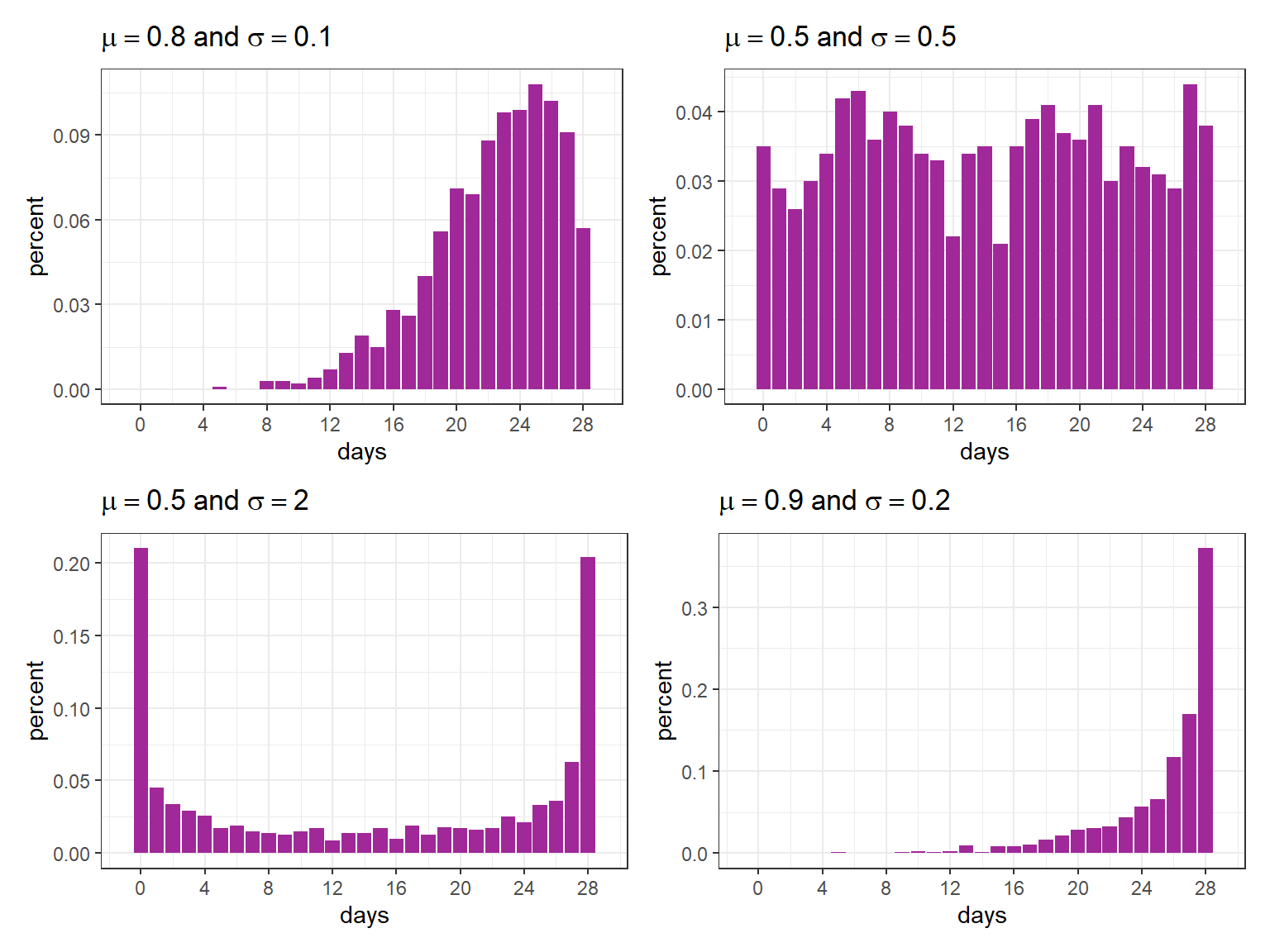
Zero Infated Beta Binomial (ZIBB)
The probabilities of the zero inflated beta binomial distribution can be described by
\[ P(Y = y|n, \mu, \sigma, \nu) = \begin{cases} \nu + (1 - \nu)P(Y_1=0|n, \mu, \sigma) \quad & \text{ if } y = 0 \\ (1 - \nu)P(Y_1=0|n, \mu, \sigma) \quad & \text{ if } y = 1, 2, 3, \dots \end{cases} \]
for \(0 < \mu < 1\), \(\sigma > 0\), \(0 < \nu < 1\), \(n\) is a positive integer and \(Y_1 \sim \text{BB}(n, \mu, \sigma)\). For this ZIBB distribution, we have
\[\text{E}(Y) = (1 - \nu)n\mu\]
\[\text{Var}(Y) = (1 - \nu)n\mu(1 - \mu)\left[1 + \frac{\sigma}{1 + \sigma}(n-1) \right] + \nu(1 - \nu)n^2\mu^2\]
We will now generate simulated data using the same parameters as the beta-binomial distribution (rBB) presented earlier, but with zero-inflation this time (rZIBB).
set.seed(21)

fig1 <- tibble(days = rBB(n = 10^3, mu =.3, sigma = .2, bd = 28)) %>%
  count(days) %>%
  mutate(percent = n / sum(n)) %>%
  ggplot(aes(days, percent)) +
    geom_col(fill = "#A02898") +
    ylim(c(0, .15)) +
    scale_x_continuous(breaks = seq(0, 30, 2)) +
    labs(title = expression(paste("BB - ")~mu==.3~and~sigma==.2))

fig2 <- tibble(days = rZIBB(n = 10^3, mu =.3, sigma = .2, nu = .1, bd = 28)) %>%
  count(days) %>%
  mutate(percent = n / sum(n)) %>%
  ggplot(aes(days, percent)) +
    geom_col(fill = "#A02898") +
    ylim(c(0, .15)) +
    scale_x_continuous(breaks = seq(0, 30, 2)) +
    labs(title = expression(paste("ZIBB - ")~mu==.3~paste(",")~sigma==.2~and~nu==.1))

fig1 / fig2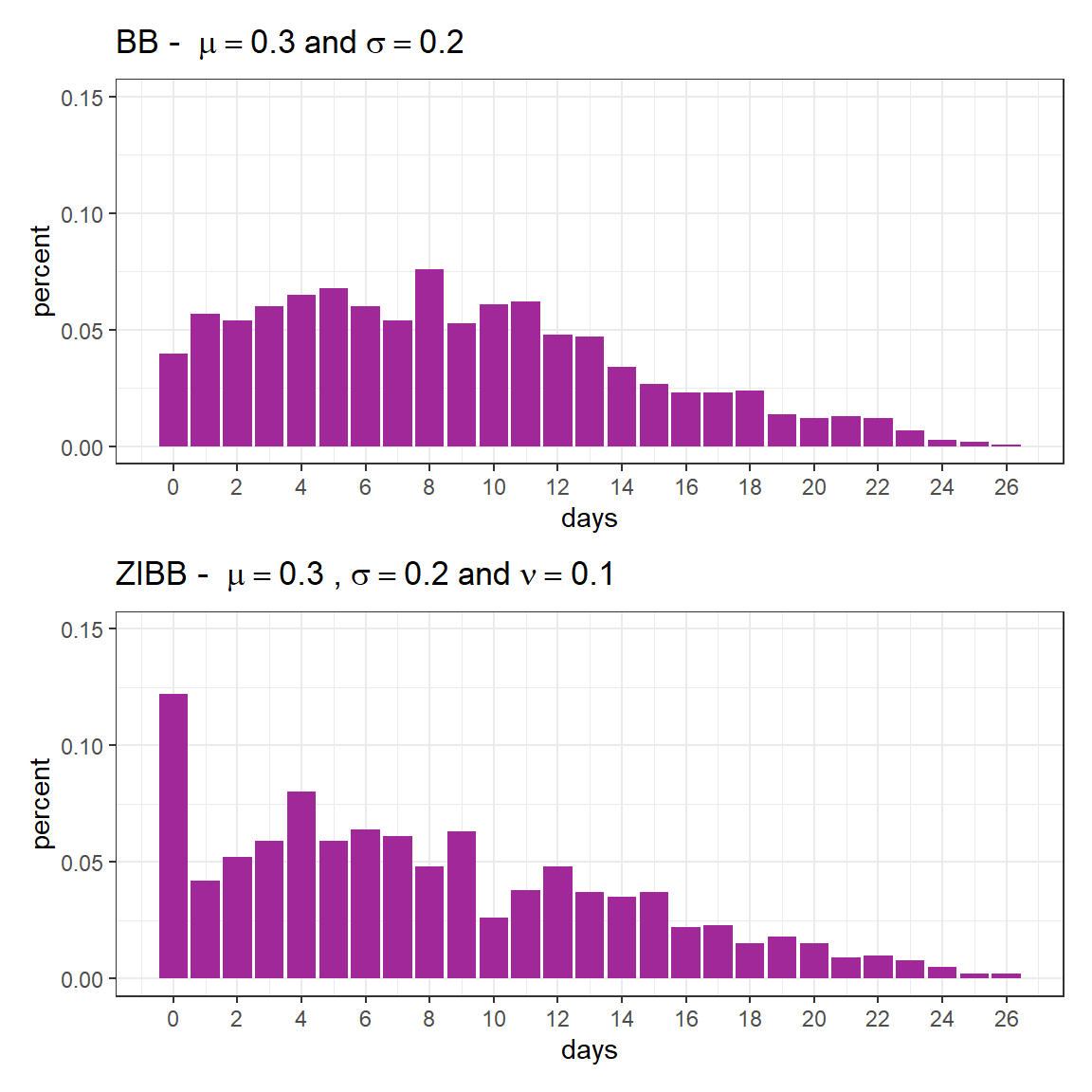
As previously mentioned, the expected value is given by
\[\text{E}(Y) = (1 - \nu)n\mu\]
(1 - 0.1)*28*.3[1] 7.56Furthermore, it is important to note that \(P(Y = 0)\) is not given by \(\nu\), but by
\[ p_0 = \nu + (1 - \nu)P(Y_1=0|n, \mu, \sigma). \]
0.1 + (1 - 0.1)*dBB(0, mu =.3, sigma = .2, bd = 28)[1] 0.1363325In the next session, we will consider a hypothetical scenario with two groups.
Simulated scenario
We will be examining a scenario involving two groups, namely the control group and intervention group. For each group, the following parameters will be taken into consideration:
- control: \(\mu = .8\), \(\sigma = .1\), \(\nu = .13\) and \(n = 28\)
- intervention: \(\mu = .5\), \(\sigma = .9\), \(\nu = .2\) and \(n = 28\)
In this case, the expected values are given by:
\[\text{E}(Y) = (1 - \nu)n\mu\]
(1 - .13) * 28 * .8 # control[1] 19.488(1 - .20) * 28 * .5 # intervention[1] 11.2Again, \(P(Y = 0)\) is not given by \(\nu\), but by
\[ p_0 = \nu + (1 - \nu)P(Y_1=0|n, \mu, \sigma) \]
.13 + (1 - .13)*dBB(0, mu =.8, sigma = .1, bd = 28)[1] 0.1300002.2 + (1 - .2)*dBB(0, mu =.5, sigma = .9, bd = 28)[1] 0.2738362Generating the simulated scenario
In order to generate the simulated data, we’ll use rZIBB.
set.seed(31)

n <- 10^3

df <- tibble(days = c(rZIBB(n, mu =.8, sigma = .1, nu = .13, bd = 28),
                      rZIBB(n, mu =.5, sigma = .9, nu = .20, bd = 28)),
             group = rep(c("control", "intervention"), each = n))
The graph below displays the proportion of observed values for each group.
df %>%
  count(group, days) %>%
  group_by(group) %>%
  mutate(percent = n / sum(n)) %>%
  ggplot(aes(days, percent)) +
    geom_col(fill = "#A02898") +
    facet_wrap(~ group, ncol = 1) +
    scale_x_continuous(breaks = seq(0, 28, 2))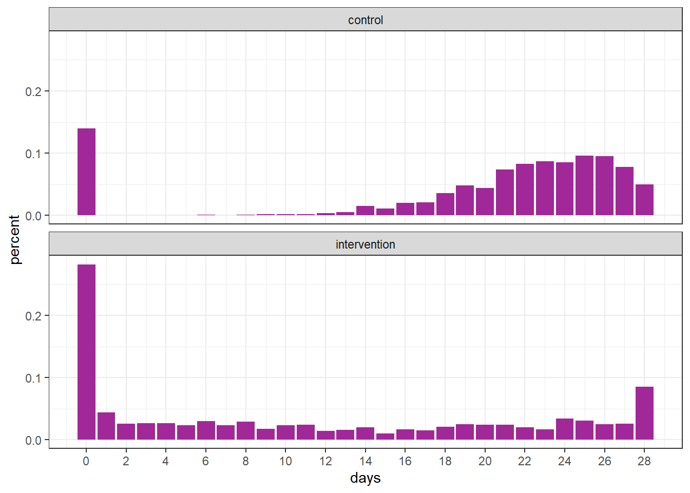
Fitting GAMLSS
fit <- gamlss(cbind(days, 28 - days) ~ group,
              sigma.formula =  ~ group,
              nu.formula =  ~ group,
              family = ZIBB(mu.link = "logit"),
              control = gamlss.control(trace = FALSE),
              data = df)

summary(fit)
******************************************************************
Family: c("ZIBB", "Zero Inflated Beta Binomial")
Call:
gamlss(formula = cbind(days, 28 - days) ~ group, sigma.formula = ~group,
nu.formula = ~group, family = ZIBB(mu.link = "logit"),
data = df, control = gamlss.control(trace = FALSE))
Fitting method: RS()
------------------------------------------------------------------
Mu link function: logit
Mu Coefficients:
Estimate Std. Error t value Pr(>|t|)
(Intercept) 1.44200 0.02980 48.39 <2e-16 ***
groupintervention -1.46888 0.08063 -18.22 <2e-16 ***
---
Signif. codes: 0 '***' 0.001 '**' 0.01 '*' 0.05 '.' 0.1 ' ' 1
------------------------------------------------------------------
Sigma link function: log
Sigma Coefficients:
Estimate Std. Error t value Pr(>|t|)
(Intercept) -2.36753 0.07053 -33.57 <2e-16 ***
groupintervention 2.30424 0.10408 22.14 <2e-16 ***
---
Signif. codes: 0 '***' 0.001 '**' 0.01 '*' 0.05 '.' 0.1 ' ' 1
------------------------------------------------------------------
Nu link function: logit
Nu Coefficients:
Estimate Std. Error t value Pr(>|t|)
(Intercept) -1.81529 0.09114 -19.919 < 2e-16 ***
groupintervention 0.43528 0.16811 2.589 0.00969 **
---
Signif. codes: 0 '***' 0.001 '**' 0.01 '*' 0.05 '.' 0.1 ' ' 1
------------------------------------------------------------------
No. of observations in the fit: 2000
Degrees of Freedom for the fit: 6
Residual Deg. of Freedom: 1994
at cycle: 10
Global Deviance: 11217.28
AIC: 11229.28
SBC: 11262.89
******************************************************************Next, we define the variables based on the estimates required to calculate the expected value.
mu_ctrl <- inv_logit(fit$mu.coefficients[[1]])
mu_int <- inv_logit(fit$mu.coefficients[[1]] + fit$mu.coefficients[[2]])

nu_ctrl <- inv_logit(fit$nu.coefficients[[1]])
nu_int <- inv_logit(fit$nu.coefficients[[1]] + fit$nu.coefficients[[2]])
In the following table, we present the sample mean, the estimated expected value using gamlss and the theoretical expected value. Note how similar these quantities are.
# observed mean
df %>%
  group_by(group) %>%
  summarise(sample_mean = mean(days)) %>%
  mutate(estimated_mean = c(mu_ctrl*28*(1 - nu_ctrl), mu_int*28*(1 - nu_int)),
         theoretical_mean = c((1 - .13)*28*.8, (1 - .20)*28*.5))
# A tibble: 2 × 4
group sample_mean estimated_mean theoretical_mean
<chr> <dbl> <dbl> <dbl>
1 control 19.5 19.5 19.5
2 intervention 11.0 11.0 11.2To check the goodness-of-fit, it is possible to use the plot function.
plot(fit)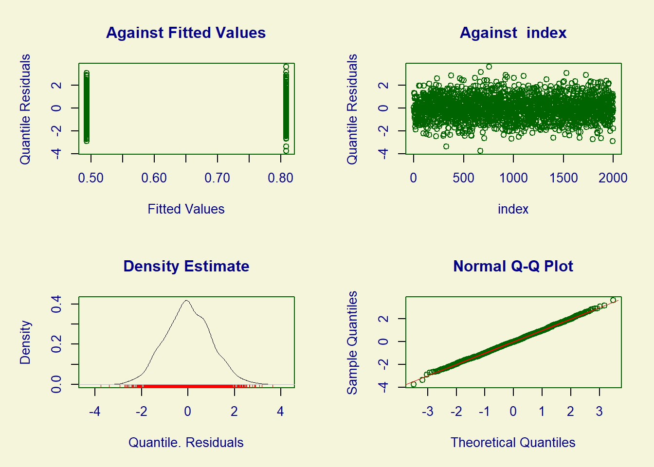
******************************************************************
     Summary of the Randomised Quantile Residuals
                           mean   =  0.001760414
                       variance   =  0.9944081
               coef. of skewness  =  0.04925325
               coef. of kurtosis  =  3.042655
Filliben correlation coefficient  =  0.9996822
******************************************************************
Bootstrap confidence intervals
One simple method to construct confidence intervals for the difference and ratio of means is by using the bootstrap techniques. In the following example, we can begin by creating an auxiliary function that performs the analysis on each bootstrap sample.
boot_estimates <- function(df_star) {

  fit <- gamlss(cbind(days, 28 - days) ~ group,
                sigma.formula =  ~ group,
                nu.formula =  ~ group,
                family = ZIBB(mu.link = "logit"),
                control = gamlss.control(trace = FALSE),
                data = training(df_star))

  mu_ctrl <- inv_logit(fit$mu.coefficients[[1]])
  mu_int <- inv_logit(fit$mu.coefficients[[1]] + fit$mu.coefficients[[2]])

  nu_ctrl <- inv_logit(fit$nu.coefficients[[1]])
  nu_int <- inv_logit(fit$nu.coefficients[[1]] + fit$nu.coefficients[[2]])

  mean_ctrl <- mu_ctrl*28*(1 - nu_ctrl)
  mean_int  <- mu_int*28*(1 - nu_int)

  tibble(outcome = c("difference", "ratio"),
         value = c(mean_int - mean_ctrl, mean_int / mean_ctrl))

}
Next, we can generate the bootstrap samples and apply the previously created function to each sample. By adopting this approach, we can analyze the distribution of these statistics, perform statistical hypothesis tests, and create confidence intervals using percentiles or other techniques. For further information on the bootstrap and bootstrap confidence intervals, please refer to (Efron and Hastie 2016).
boot_obs <- df %>%
  rsample::bootstraps(times = 10^3) %>%
  mutate(results = map(splits, boot_estimates)) %>%
  unnest(cols = results)
boot_obs %>%
ggplot(aes(value, after_stat(density))) +
geom_histogram(fill = "#A02898", color = "white") +
facet_wrap(~ outcome, scales = "free", ncol = 1)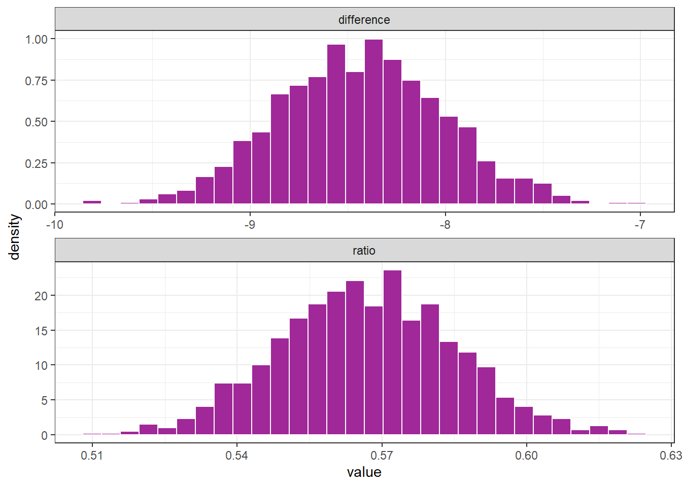
boot_obs %>%
  group_by(outcome) %>%
  summarise(perc_025 = quantile(value , .025),
            perc_975 = quantile(value , .975))
# A tibble: 2 × 3
outcome perc_025 perc_975
<chr> <dbl> <dbl>
1 difference -9.23 -7.59
2 ratio 0.532 0.604Estimation of percentiles through theoretical distribuition
To confirm the proximity between the percentiles obtained using bootstrap and the percentiles obtained through the theoretical distribution, we can utilize the following code:
set.seed(5)

rand_sample <- function(n) {

  ctrl <- mean(rZIBB(n, mu =.8, sigma = .1, nu = .13, bd = 28))
  int  <- mean(rZIBB(n, mu =.5, sigma = .9, nu = .20, bd = 28))

  tibble(outcome = c("difference", "ratio"),
         value = c(int - ctrl, int / ctrl))
}


tibble(b = 1:10^3) %>%
  mutate(data = map(b, ~rand_sample(n = 10^3))) %>%
  unnest(data) %>%
  group_by(outcome) %>%
  summarise(perc_025 = quantile(value , .025),
            perc_975 = quantile(value , .975))
# A tibble: 2 × 3
outcome perc_025 perc_975
<chr> <dbl> <dbl>
1 difference -9.16 -7.54
2 ratio 0.536 0.608Note that the values obtained are remarkably similar to the bootstrap values derived from the previously generated single sample. However, further investigation is recommended in each scenario to verify this behavior.
Truncated distributions
As an illustration of a truncated function, we will use the gamma distribution.
Gamma distribution
To generate data from a gamma distribution, we can use the rGA function.
df <- tibble(days = rGA(n = 1000, mu = 10, sigma = .8))

df %>%
  ggplot(aes(days, after_stat(density))) +
    geom_histogram(color = "white", fill = "#A02898") +
    geom_vline(xintercept = 15, linetype = 2,
               color = "#2a9d8f", linewidth = 1)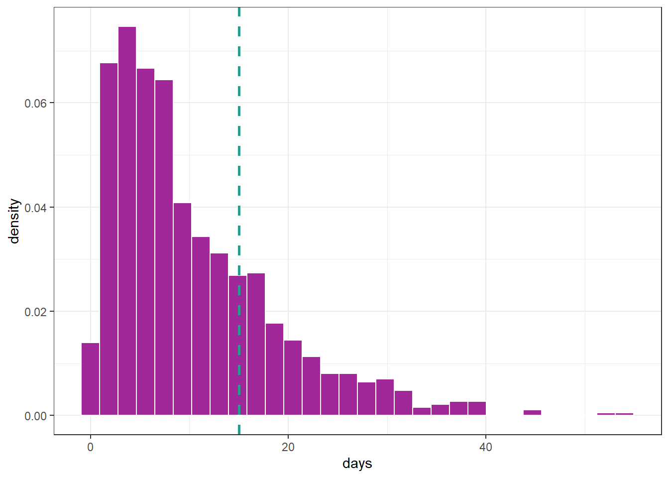
Suppose we want to focus on the gamma distribution presented in the previous graph but only for values up to 15, i.e., the data falls within the interval \((0, 15]\). To achieve this, we can create a truncated distribution that specifies the distribution family, the truncation value, and whether it will be truncated on the left, right, or both sides. For instance, in this example, we can use the following settings:
gen.trun(par = c(15), type = "right", family = GA(), name = "trunc")A truncated family of distributions from GA has been generated
and saved under the names:
dGAtrunc pGAtrunc qGAtrunc rGAtrunc GAtrunc
The type of truncation is right
and the truncation parameter is 15 We now have an rGAtrunc function to generate data from a range truncated by \(15\). Let’s compare the usual distribution to the truncated distribution:
set.seed(15)

# GA
df <- tibble(days = rGA(n = 10^3, mu = 10, sigma = .8))

fig1 <- df %>%
  ggplot(aes(days, after_stat(density))) +
  geom_histogram(color = "white", fill = "#A02898") +
  labs(title = expression(paste("GA (")~mu==.8~and~sigma==.8~paste(")"))) +
  scale_x_continuous(limits = c(-2, 70)) +
  scale_y_continuous(limits = c(0, .1))

# GAtrunc
df <- tibble(days = rGAtrunc(n = 10^3, mu = 10, sigma = .8))

fig2 <- df %>%
  ggplot(aes(days, after_stat(density))) +
  geom_histogram(color = "white", fill = "#A02898") +
  labs(title = expression(paste("GAtrunc (")~mu==.8~paste(",")~sigma==.8~paste("and truncated at 15)"))) +
  geom_vline(xintercept = 15, linetype = 2, color = "#2a9d8f", linewidth = 1) +
  scale_x_continuous(limits = c(-2, 70)) +
  scale_y_continuous(limits = c(0, .1))


fig1 / fig2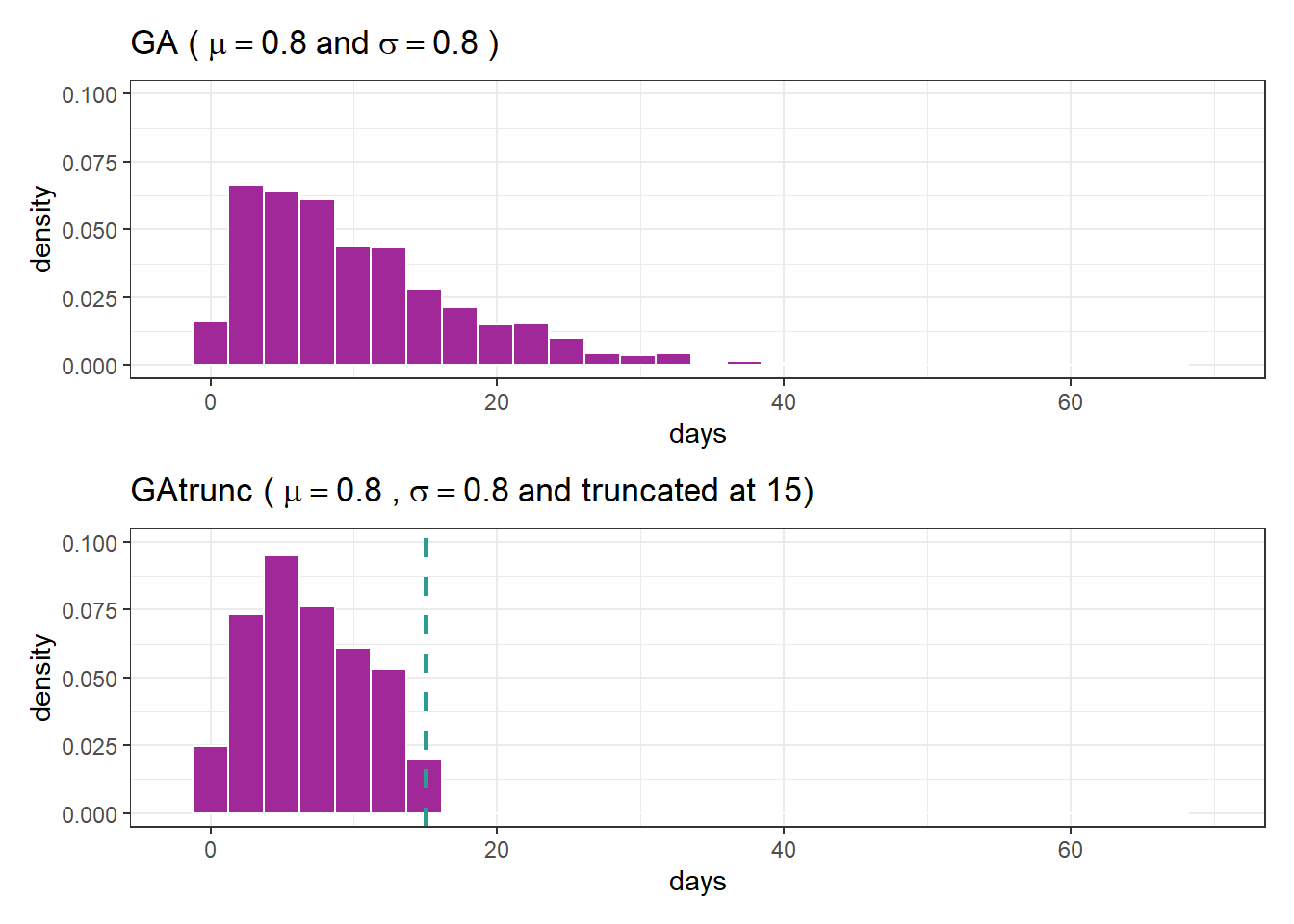
Fitting GAtrunc
Now we will fit a model considering the previously defined truncated distribution.
fit_tr <- gamlss(days ~ 1, family = GAtrunc,
                 control = gamlss.control(trace = FALSE),
                 data = df)

summary(fit_tr)
******************************************************************
Family: c("GAtrunc", "right truncated Gamma")
Call: gamlss(formula = days ~ 1, family = GAtrunc, data = df,
control = gamlss.control(trace = FALSE))
Fitting method: RS()
------------------------------------------------------------------
Mu link function: log
Mu Coefficients:
Estimate Std. Error t value Pr(>|t|)
(Intercept) 2.39890 0.08297 28.91 <2e-16 ***
---
Signif. codes: 0 '***' 0.001 '**' 0.01 '*' 0.05 '.' 0.1 ' ' 1
------------------------------------------------------------------
Sigma link function: log
Sigma Coefficients:
Estimate Std. Error t value Pr(>|t|)
(Intercept) -0.22320 0.02901 -7.695 3.39e-14 ***
---
Signif. codes: 0 '***' 0.001 '**' 0.01 '*' 0.05 '.' 0.1 ' ' 1
------------------------------------------------------------------
No. of observations in the fit: 1000
Degrees of Freedom for the fit: 2
Residual Deg. of Freedom: 998
at cycle: 13
Global Deviance: 5345.843
AIC: 5349.843
SBC: 5359.658
******************************************************************We can assess the model’s goodness of fit using the plot function. We can examine the symmetry of the residuals and ensure that the points on the graph align with the reference line.
plot(fit_tr)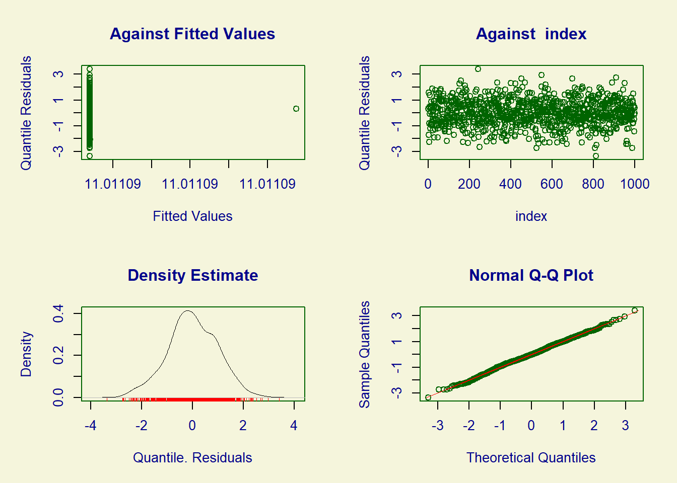
******************************************************************
          Summary of the Quantile Residuals
                           mean   =  -0.003691478
                       variance   =  0.9857485
               coef. of skewness  =  -0.05881383
               coef. of kurtosis  =  3.061488
Filliben correlation coefficient  =  0.9991239
******************************************************************
# mu teórico = 10
exp(fit_tr$mu.coefficients)(Intercept)
11.01109 # sigma teórico = .8
exp(fit_tr$sigma.coefficients)(Intercept)
0.7999561 Next, we will present fits using both the standard gamma distribution and the truncated gamma distribution.
fit_ga <- gamlss(days ~ 1, family = GA,
                 control = gamlss.control(trace = FALSE),
                 data = df)

df %>%
  ggplot(aes(days)) +
  geom_histogram(aes(y = after_stat(density)), color = "black", fill = NA) +
  stat_function(aes(color = "GAtrunc - estimation"), linewidth = 1,
                fun = dGAtrunc, args = list(mu = exp(fit_tr$mu.coefficients),
                                       sigma = exp(fit_tr$sigma.coefficients))) +
  stat_function(aes(color = "GAtrunc - theoretical"), linewidth = 1,
                fun = dGAtrunc, args = list(mu = 10, sigma = .8)) +
  stat_function(aes(color = "GA - estimation"), linewidth = 1,
                fun = dGA, args = list(mu = exp(fit_ga$mu.coefficients),
                                            sigma = exp(fit_ga$sigma.coefficients))) +
  scale_color_manual(values = c("GAtrunc - estimation" = "blue",
                                "GAtrunc - theoretical" = "red",
                                "GA - estimation" = "#2a9d8f")) +
  labs(color = NULL, title = "Adjusted with truncated GA") +
  theme(legend.position = "top")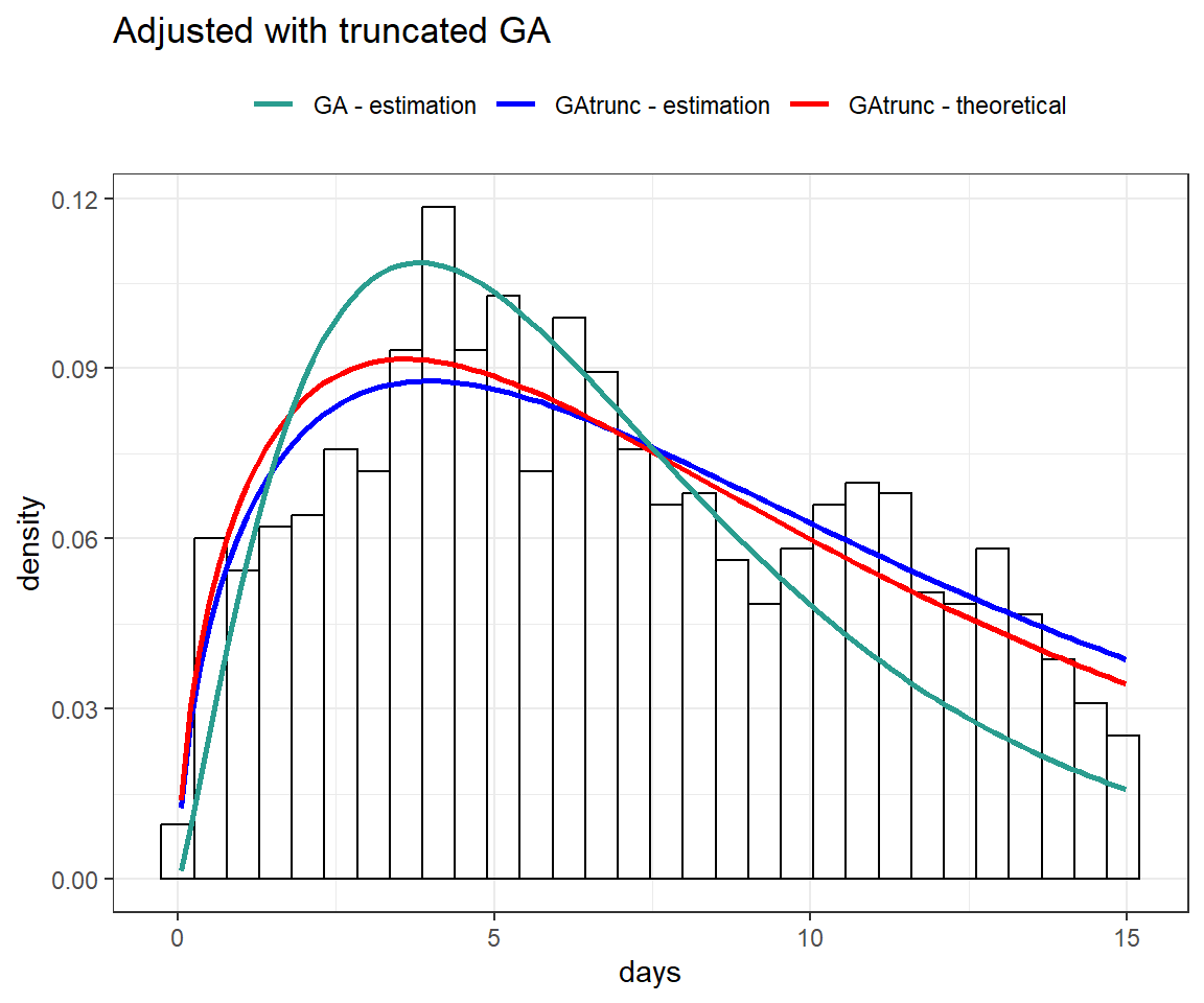
Useful links
- sites
- books
- vignetes
- videos
- paper/theses/dissertations
- Costa, Á. C. de L., Oliveira, A. D. M. de ., Caraciolo, J. P. S., Lucena, L. R. R. de ., & Leite, M. L. de M. V.. (2022). A GAMLSS approach to predicting growth of Nopalea cochenillifera Giant Sweet clone submitted to water and saline stress. Acta Scientiarum. Agronomy, 44(Acta Sci., Agron., 2022 44), e54939. https://doi.org/10.4025/actasciagron.v44i1.54939
- THOMAS, Gustavo. GAMLSSs with applications to zero inflated and hierarquical data. doi:10.11606/D.11.2018.tde-06042018-150012. Piracicaba: Escola Superior de Agricultura Luiz de Queiroz, University of São Paulo, 2017. Master’s Dissertation in Estatística e Experimentação Agronômica
References
Efron, Bradley, and Trevor Hastie. 2016. Computer Age Statistical Inference: Algorithms, Evidence, and Data Science. 1st ed. USA: Cambridge University Press.
Rigby, R. A., and D. M. Stasinopoulos. 2005. “Generalized Additive Models for Location, Scale and Shape.” Journal of the Royal Statistical Society: Series C (Applied Statistics) 54 (3): 507–54. https://doi.org/https://doi.org/10.1111/j.1467-9876.2005.00510.x.